Autoencoders & Decoders using Keras

Project Overview

This is a comprehensive, modular Python application implementing multiple autoencoder architectures for image compression, reconstruction, denoising, similarity search, and image morphing. It was upgraded from an old Jupyter notebook into a professional, production-quality codebase with a single CLI entry point supporting five operational modes.

The project covers progressive complexity: from a simple linear PCA-style autoencoder, through a deep convolutional architecture, to a noise-robust denoising variant. Each model shares the same interface and can be used for downstream applications like image retrieval via k-NN in latent space and smooth image morphing via latent interpolation.

Why I Built This

I had an old Jupyter notebook that implemented autoencoders using TensorFlow 1.x. It worked, but it was a single monolithic file that was hard to reproduce, extend, or share. I wanted to rebuild it as a proper Python application: modular, documented, typed, and runnable with a single command.

Beyond the refactoring goal, this project is designed as an educational resource. It shows how autoencoders work at three levels of complexity, demonstrates real applications (retrieval and morphing), and serves as a reference for anyone learning about latent space representations in deep learning.

The Core Idea

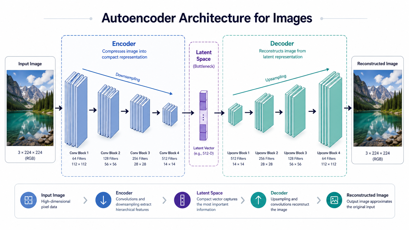
An autoencoder is a neural network that learns to compress data into a small representation and then reconstruct the original from that compressed form. The bottleneck forces the network to learn what is truly important about the input - it cannot memorize, it must understand.

Input Image (32×32×3 = 3,072 numbers)
        ↓
    [ENCODER]
    Compresses information
        ↓
Latent Code (32 numbers) ← The "essence" of the image
        ↓
    [DECODER]
    Reconstructs from code
        ↓
Output Image (32×32×3 = 3,072 numbers)

Loss = ||Input - Output||²  →  minimize reconstruction error

The key insight is that the latent space (the space of all compressed codes) develops useful properties: nearby codes correspond to similar images, the space is continuous, and you can interpolate smoothly between any two images by interpolating their codes.

Key Features

Architecture Details

PCA Autoencoder (Linear Baseline)

The simplest architecture: flatten the image, project down to a 32-dimensional code through a single dense layer, then project back up. No activation functions, pure linear transformations. This is mathematically equivalent to PCA but learned through backpropagation.

Input (32×32×3)
      ↓
   Flatten → (3,072)
      ↓
   Dense(32) ← Bottleneck (96× compression)
      ↓
   Dense(3,072)
      ↓
   Reshape → (32×32×3)
      ↓
Output (32×32×3)

Parameters: ~100,000 | Training: ~2 min (CPU)

Convolutional Autoencoder (Production Quality)

A deep CNN that learns hierarchical features through four convolutional blocks with progressive filter growth (32 → 64 → 128 → 256). The decoder mirrors the encoder using transpose convolutions for learned upsampling. This achieves the same 96× compression ratio as PCA but captures non-linear patterns for dramatically better reconstruction.

ENCODER:
Input (32×32×3)
  → Conv2D(32, 3×3) + ReLU + MaxPool(2×2)  → (16×16×32)
  → Conv2D(64, 3×3) + ReLU + MaxPool(2×2)  → (8×8×64)
  → Conv2D(128, 3×3) + ReLU + MaxPool(2×2) → (4×4×128)
  → Conv2D(256, 3×3) + ReLU + MaxPool(2×2) → (2×2×256)
  → Flatten → Dense(32) + ReLU  ← Bottleneck

DECODER:
Dense(1024) + ReLU → Reshape (2×2×256)
  → Conv2DTranspose(128, 3×3, stride=2) + ReLU → (4×4×128)
  → Conv2DTranspose(64, 3×3, stride=2) + ReLU  → (8×8×64)
  → Conv2DTranspose(32, 3×3, stride=2) + ReLU  → (16×16×32)
  → Conv2DTranspose(3, 3×3, stride=2)          → (32×32×3)

Parameters: ~800,000 | Training: ~20 min (CPU) / ~5 min (GPU)

What Each Encoder Layer Learns

How It Works

1. Data loading: The STL-10 dataset is automatically downloaded and preprocessed. Images are resized to 32×32×3 and normalized to [0, 1].
2. Model building: Each architecture returns three models - the full autoencoder, the encoder alone, and the decoder alone - sharing weights. This allows independent use of each component.
3. Training: The autoencoder is trained to minimize MSE between input and output. Input equals output (unsupervised). Callbacks handle early stopping, learning rate scheduling, and checkpointing.
4. Encoding: After training, the encoder maps any image to a compact latent code. Similar images produce similar codes, which enables downstream applications.
5. Retrieval: All training images are encoded once. Given a query image, its code is compared against all stored codes using k-NN to find the most similar images.
6. Morphing: Two images are encoded, their codes are linearly interpolated at N steps, and each intermediate code is decoded to produce a smooth visual transition.
7. Denoising: Gaussian noise is added to inputs each epoch during training, but the target remains the clean original. This forces the network to learn features that ignore noise.

Core Code Snippets

Building the convolutional autoencoder

The build function returns three separate models that share weights. This is the key pattern that enables using the encoder and decoder independently after training.

from models import build_convolutional_autoencoder

autoencoder, encoder, decoder = build_convolutional_autoencoder(
    input_shape=(32, 32, 3),
    code_size=32,
    filters=(32, 64, 128, 256)
)

autoencoder.compile(optimizer='adamax', loss='mse')
autoencoder.fit(X_train, X_train, epochs=25, batch_size=32)

Image retrieval via latent space k-NN

Once images are encoded, finding similar images is just a nearest neighbor search in the 32-dimensional latent space. This is orders of magnitude faster than comparing raw pixels.

from image_retrieval import ImageRetrieval

retrieval = ImageRetrieval(encoder)
retrieval.index_images(X_train)  # Encode all images once

# Find 5 most similar images to a query
distances, similar = retrieval.find_similar(query_image, n_neighbors=5)

Image morphing via latent interpolation

Smooth transitions between images are possible because the latent space is continuous. Linearly interpolating between two codes produces semantically meaningful intermediate images.

from image_morphing import interpolate_images

# Generate 7-step morph between two images
morphed = interpolate_images(
    image1, image2,
    encoder, decoder,
    n_steps=7
)

# How it works internally:
# z1 = encoder(image1), z2 = encoder(image2)
# z_interp = α×z1 + (1-α)×z2 for α ∈ [0, 1]
# morphed[i] = decoder(z_interp[i])

Denoising training loop

The denoising autoencoder adds fresh noise each epoch so the network never memorizes specific noise patterns. The target is always the clean original image.

from utils import apply_gaussian_noise

for epoch in range(25):
    X_train_noisy = apply_gaussian_noise(X_train, sigma=0.1)
    autoencoder.fit(X_train_noisy, X_train, epochs=1)
    # Key: noisy input → clean target

Performance & Metrics

Model Comparison

Usage

python main.py --mode pca \
  --epochs 15 --code-size 32

python main.py --mode convolutional \
  --epochs 25 --code-size 32

python main.py --mode denoising \
  --epochs 25 --noise-sigma 0.1

python main.py --mode retrieval \
  --model-path saved_models \
  --n-queries 3 --n-neighbors 5

python main.py --mode morphing \
  --model-path saved_models \
  --n-pairs 5 --n-steps 7

pip install -r requirements.txt
python example_usage.py

Project Structure

Autoencoders-Decoders-using-Keras/
│
├── main.py                    # CLI entry point (5 modes)
├── config.py                  # Configuration management
├── example_usage.py           # Quick 2-minute demo
│
├── models/                    # Autoencoder architectures
│   ├── pca_autoencoder.py            # Linear (PCA-style)
│   ├── convolutional_autoencoder.py  # Deep CNN
│   └── denoising_autoencoder.py      # Noise-robust
│
├── utils/                     # Reusable utilities
│   ├── data_loader.py               # Dataset handling
│   ├── visualization.py             # Plotting tools
│   └── noise.py                     # Noise generation
│
├── image_retrieval.py        # Similarity search
├── image_morphing.py         # Image interpolation
│
├── requirements.txt          # Dependencies
└── README.md                 # Complete documentation

Tech Stack

The Upgrade: Old Notebook → Modern Application

My Contribution

I designed and built this project end to end:

• Upgraded the entire codebase from a single TF 1.x notebook to a modular TF 2.13+ application with 16 professional files
• Designed and implemented three autoencoder architectures with progressive complexity (PCA → CNN → Denoising)
• Built the image retrieval system using k-NN in latent space for fast semantic similarity search
• Implemented image morphing via latent space interpolation with configurable step counts
• Created the unified CLI entry point supporting all five modes with full argument customization
• Wrote comprehensive documentation covering theory, architecture, usage, and mathematical foundations

Challenges & Learnings

Linear vs non-linear compression quality
The PCA autoencoder shows exactly what you lose with linear compression - it captures global structure but misses textures, fine edges, and complex patterns. Comparing its output side by side with the convolutional autoencoder makes the value of non-linear feature learning immediately visible and intuitive.

Latent space continuity is not guaranteed
Unlike variational autoencoders, standard autoencoders do not explicitly enforce continuity in latent space. Morphing works because the training distribution is dense enough, but there can be "holes" in latent space where decoded outputs look unrealistic. Understanding this limitation was key to setting correct expectations for the morphing application.

Denoising requires careful noise calibration
Too little noise (sigma < 0.05) and the network barely learns denoising - it can reconstruct clean images without ignoring noise. Too much noise (sigma > 0.3) and reconstruction quality degrades because the input is too corrupted to extract structure from. The sweet spot (0.1-0.2) produces genuinely robust features.

Code size vs reconstruction quality trade-off
A code size of 32 achieves 96× compression but visibly loses fine detail. Increasing to 128 dramatically improves quality at the cost of less compression (24×). This trade-off is fundamental to representation learning and becomes a design decision based on the downstream application.

Future Improvements

• Add a Variational Autoencoder (VAE) with KL divergence regularization for a properly structured latent space
• Implement GAN-based decoder training for sharper reconstructions (adversarial autoencoder)
• Support higher resolution inputs (64×64, 128×128) with deeper architectures
• Add latent space visualization using t-SNE or UMAP to show cluster structure
• Implement progressive training where code size gradually decreases during training
• Add a Streamlit or Gradio demo for interactive exploration without command-line setup

Closing Note

This project is fully open source and designed to be both educational and practical. It demonstrates how autoencoders work at multiple levels of complexity, shows real-world applications beyond simple reconstruction, and serves as a clean reference implementation for anyone learning about latent representations in deep learning.

If you are studying representation learning, working on image compression, or just want to understand how neural networks learn to "summarize" images into compact codes, this project covers the full pipeline from theory to working applications.